
Hello guys! After covering Pandas and Naive Bayes algorithm, it's time to shift the gear to building models in Machine Learning and the simplest among these algorithms is the Linear Regression Model.
Introduction:
The Linear Regression model is a discriminative type algorithm, which is a class of machine learning algorithm to relate the dependency of the unobserved (dependent) variable, i.e 'y' on the observable (independent) variables i.e 'xi'. Unlike generative models, it doesn't allow the user to generate samples from the joint distribution of the observed and target variable. Linear regression is a supervised learning algorithm, i.e it requires the model to be trained with labelled dataset so that it can make predictions.
What is a Regression Model?
A regression model is a method to determine the average value of the dependent variable, given the independent variables. This is determined by a connecting equation for the model. A regression model is not used to classify something into classes, rather it is used for prediction purposes like housing price prediction, population statistics etc. Basically, given the result of some data, you have to predict what the result of a new data-point can be.
A regression model consists of the following parameters:
- The dependent variable (y)
- The independent variables (xi)
- The unknown constants (b).
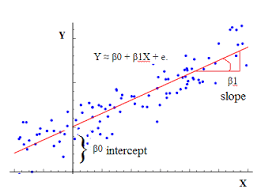
When all these are connected by a linear equation, it is known as a linear regression model. Suppose we have a dependent variable y, and three independent variables x1, x2, and x3; they can be related by the equation: Y = b0+b1.x1+b2.x2+b3.x3+e, where e is the random error constant(Basically, the error represents everything that the model does not have into account. And why is that? Because it would be extremely unlikely for a model to perfectly predict a variable, as it is impossible to control every possible condition that may interfere with the response variable. The errors may also include reading or measuring inaccuracies.)
The thing is, we don't know the values of b1, b2, and b3. Hence, we need a method to find out suitable values for the unknown constants, such that there is a minimum error during the prediction procedure. This method is known as the Gradient Descent. There are various types of Gradient Descent algorithm, but here we are going to work with Stochastic Gradient Descent. Other types of Gradient Descent algorithms are: Batch Gradient Descent and LBFGS, to name a few.
Gradient Descent:
The gradient descent is an optimisation algorithm, i.e it works towards finding the minimum value of the specified function. Confusing to think how this finds the optimal value of constants, right? Well, This works out in the following way. We randomly initialise the values for the constants, and then we make a function known as a cost function, which would be the square of the difference of the predicted and the actual values of the dependent variable, i.e C(x) = (Y-y)². Now, out task is to minimise this cost function, an we do so by finding out its differential, and then subtracting it from the value of b. Now, this is getting a bit overwhelming, so we have written a separate article which explains these things in a bit more details. Click here to read it.
This is what a standard batch gradient descent algorithm would do. The Stochastic gradient descent would do all this in an iterative manner, i.e. it would consider one data at a time as opposed to the batch gradient descent, which takes the sum of all the data in the dataset for minimisation purpose.
How to put all this together?
Now that we have a basic framework of how the linear regression model works, we will start coding the model. We will be using a housing price dataset to work with, click here to get the dataset. If you want just the main code, you can skip to the bottom of the page or learn to code the hard way (the best :P).
All the codes for this tutorial can be found here.
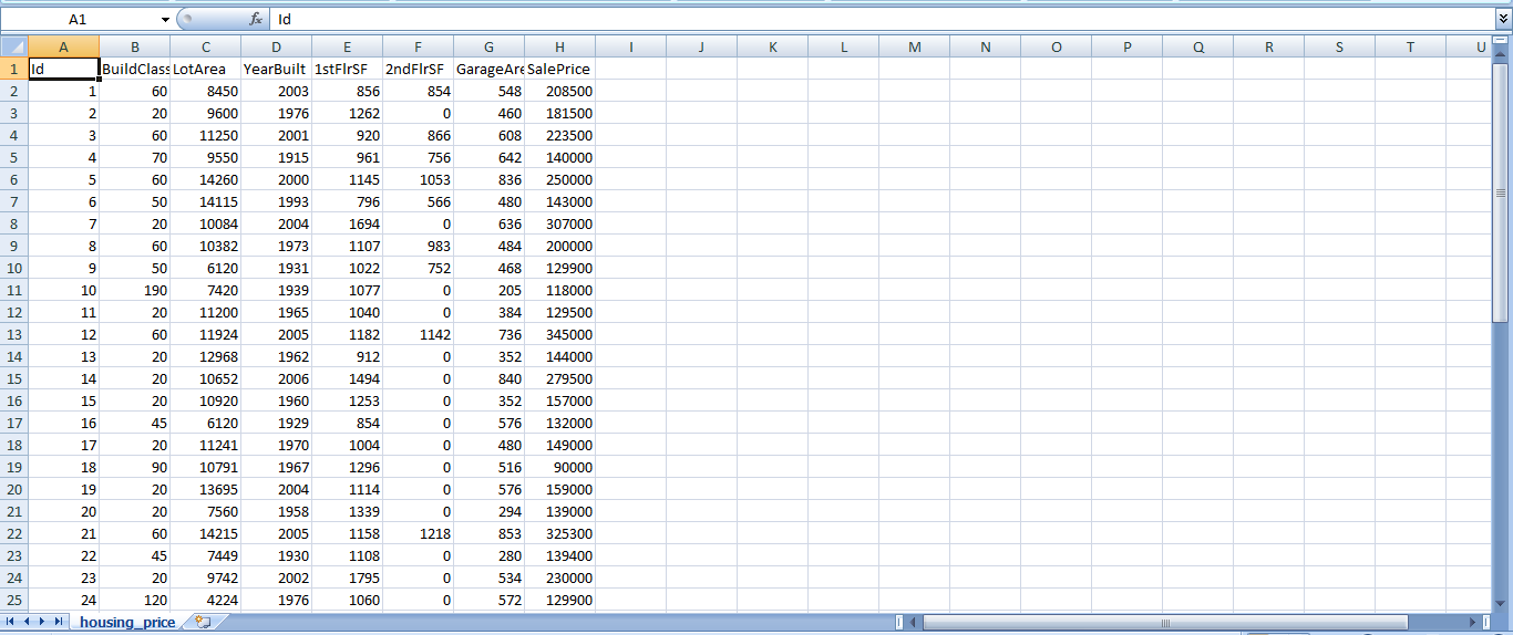 This is how our dataset looks like.
The first task that needs to be done before any algorithm or model is implemented is to pre-process the data that we have. One thing that we have to make sure is that the data is normalized. It means that all the data needs to be in same range as for instance, 0 <= x <= 1, so that data can be compared and the weights of the input instances are comparable. Below is the implementation of the normalizer that we will be using later.
#To find min and max of the given attributes

def find(data):
    minmax=[]
    for i in range(len(data[0])):
        r=[row[i] for row in data]
        min_val=min(r)
        max_val=max(r)
        minmax.append([min_val,max_val])
    return minmax
This is the supporting function for the normalizer which is executed as follows:
def normalizer(data,minmax): #for data scaling
    for i in range(len(data)):
        for j in range(len(data[0])):
            data[i][j]=(data[i][j]-minmax[j][0])/(minmax[j][1]-minmax[j][0])
    return data
This function normalizes the input data values for all the instances. We have already explained the SGD algorithm optimises the model by updating the coefficients of Linear Regression expression iteratively for a set number of epochs and a learning rate ( Details about epochs and learning rate has been explained here ).
def coefficient_LR(train, learning_rate, n_epoch):
    coeff= [0.0 for i in range(len(train[0]))] # to make a list for the number of coefficient and initialise them to zero.
    for epoch in range(n_epoch):
        for row in train:
            pred=predict(row,coeff)
            error=pred-row[-1]
            coeff=coeff-learning_rate*error
            for i in range(len(row)-1):
                coeff[i+1]-=learning_rate*error*row[i]
    return coeff
This function predicts the coefficients of the expression at each step using the predict function below and then updates the coefficient value for the next iteration.
def predict(row,coeff):
    pred=coeff[0]
    for i in range(len(row)-1):
        pred+=coeff[i+1]*row[i]
    return pred
Now that we are done with the prediction of coefficients for the epochs. It's time to make some data predictions. Here's how you can execute the Linear Regression model.
def linear_regression(train,test,learning_rate,n_epochs):
    predictions=[]
    coeff=coefficient_LR(train,learning_rate,n_epochs)
    for row in test:
        pred=predict(row,coeff)
        predictions.append(pred)
    return predictions
Okay, so everything is set. We should now go ahead and train the model as well as test its predictions on some data. We make a split function, similar to the one used in the Naive Bayes tutorial, and then we call each functions one by one. Here's how we do it:
import random
def split_dataset(data,sp_ratio):
    orig= data
    train_len=(int)(len(data)*sp_ratio)
    train_set=[]
    while(len(train_set)<=train_len):
        index = random.randrange(len(data))
        rowhere=(list)(data[index:index+1].values.flatten())
        train_set.append(rowhere)
        data.drop(data.index[index],inplace=True)
    test_set=data.values.tolist()
    return [train_set,test_set]
There goes our split function. Now we'll call every function one by one:
import pandas as pd
import numpy as np
df=pd.read_csv("C:\\Users\\hp\\Desktop\\housing_price.csv")
df.drop(df.columns[0],axis=1,inplace=True)
train,test=split_dataset(df,0.8)
minmax_train=find(train)
minmax_test=find(test)
ntrain=normalizer(train,minmax_train)
ntest=normalizer(test,minmax_test)
learning_rate=0.01
n_epochs=500
predictions=linear_regression(ntrain,ntest,learning_rate,n_epochs)
npredictions=[]
for pred in predictions:
    pred=pred*(minmax_test[-1][1]-minmax_test[-1][0])+minmax_test[-1][0]
    npredictions.append(pred)
print(npredictions)
So, let's check the accuracy of our model, shall we?
First we need a function for the accuracy function:
def accuracy(test,predictions):
    error=0.0
    i=0
    for row in test:
        a=np.abs(test[i][-1]-predictions[i])
        i+=1
        error+=a
    error=(error/len(predictions))*100
    accuracy=100-error
    return accuracy
Now, we will call the function and check how efficiently we have coded the model:
accuracy=accuracy(ntest,predictions)
print(accuracy)
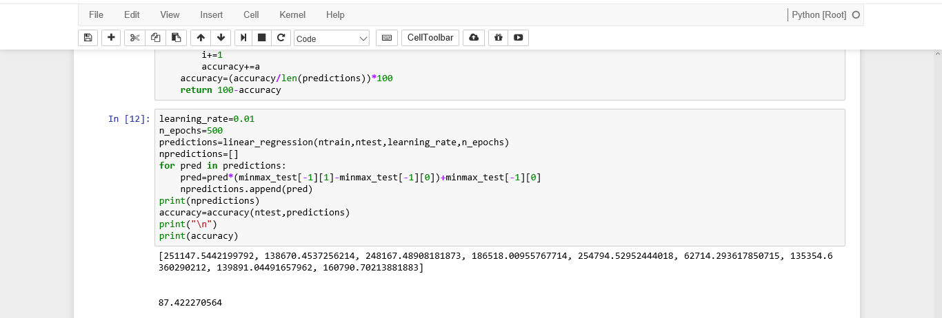 This is the output of our model
87%…that's a good accuracy for a small dataset. You guys should check the model by using the full dataset, and tweak the code as required. You can get the full dataset here.
Now, its time for the final part of the article, where we'll learn how to use the inbuilt library function for the Linear Regression model. Here we go:
sf=df.values.tolist()
x=[]
y=[]
temp=[]
for i in range(len(sf)):
    for j in range(1,len(sf[i])-1):
        temp.append(sf[i][j])
    x.append(temp)
    temp=[]
    y.append(sf[i][-1])
X_train, X_test, Y_train, Y_test = train_test_split(x, y, test_size=0.33, random_state=1)

from sklearn.linear_model import LinearRegression
clf=LinearRegression()
clf.fit(X_train,Y_train)
print(clf.predict(X_test))
print(clf.score(X_test,Y_test)*100)
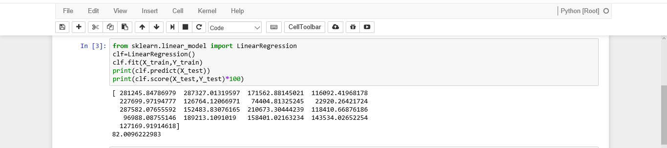 The output for the inbuilt library functions.
Viola!! Our model has fared better than the inbuilt model in terms of accuracy(:p), but that might be just because of using random data for testing.
That's all for today. Do mail us your queries and we'll be more than happy to answer them. We'll be back soon with another model, known as the Logistic Regression, well, but this algorithm is quite different than some Regression model. Why? We shall find that out in the next tutorial. Until then, Ciao!