
Hello everyone! We are back with a brand new tutorial on one of the most popular Machine Learning algorithm, the Naive Bayes algorithm.
Introduction:-
The Naive Bayes algorithm is a generative type Machine Learning algorithm, which, as its name suggests, generates a model for the various classes of data into which our dataset needs to be classified into, unlike a discriminative algorithm, which creates a boundary between the different classes into which data needs to be separated. Also, it is a supervised algorithm, i.e we need to to train the model using a dataset to make predictions. So, how does this algorithm work?
Well, this algorithm makes use of Bayes theorem from our good ol' probability chapter from high school, to create models for the various data classes. Broadly speaking, there are three kinds of Naive Bayes algorithm:
- Gaussian Naive Bayes
- Multinomial Naive Bayes
- Bernoulli Naive Bayes.
Here we are going to cover Gaussian Naive Bayes algorithm, which assumes all the data in the dataset are continuous (not discrete) and follow a normal distribution.
So, what are Bayes Theorem and Gaussian Distribution?
Bayes Theorem is a method to describe the probability of occurrence of an event provided we have some information which is related to the occurrence of the event. It is given by the following formula:
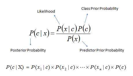
Here, P(c|x) is the probability of occurrence of an event 'c' given the conditions 'x'; P(x|c) is the probability of occurrence of 'x' given the conditions 'c', and P(c) and P(x) are the probabilities of occurrence of 'x' and 'c' independently.
Now, if for a single class 'c', we have multiple attributes X={x1,x2,…..,xn}; then the Posterior probability i.e P(c|X) is the multiplication of all the Likelihoods of attributes x1,x2,….,xn. That is what the second line in the formula states. We will be using this method to calculate the probabilities of the various classes to which a certain set of attributes may belong, and the class with the highest Posterior Probability is our prediction result.
If our data is continuous, then we apply Gaussian distribution formula to find the Posterior Probability of the classes. The Gaussian distribution is give by the following formula:
p(x=v|c) = (1/√(2πσ²c)) * e^(-(v-μc)²/(2σ²c))
Here, P(v|c) is the Likelihood for any v∈X as stated above. The value μc and σc are the mean of the values of attributes for class 'c' and variance of the attributes for the class 'c'.
So, basically Bayes theorem helps us calculate conditional probability with the Gaussian distribution helping us get the Likelihood values.
How do we get about using it?
These all mathematical things might seem a little overwhelming to you, but don't worry! We've got you covered. We'll help you how to build our predictive model step-by-step for our dataset on t20 cricket matches, which can be found here.
All the codes of this tutorial can be found here.
First of all, we need to clean up our dataset, and for that we are going to use our good friend, the pandas library. Here is the code for doing it:
import pandas as pd
import numpy as np
import scipy as sp
df1=pd.read_csv("C:\\Users\\hp\\datasets\\t20.csv")
dfx=df1[df1.Innings1Team==df1.Winner]
dfy= df1[df1.Innings1Team!=df1.Winner]
dfx['Winner']=0
dfy['Winner']=1
df1=pd.concat([dfx,dfy],ignore_index=True)
df1.replace(['Abu Dhabi','Adelaide','Bangalore','Birmingham','Cape Town'],[0,1,2,3,4], inplace=True)
original=df1
del df1['Innings1Team'] #as we no longer need the name of the team
print (df1)
Here, we basically segregate our dataset according to the team which wins the game. Also we need to set result as 0 or 1. Next, we put the values of the stadiums as 1 ,2, 3, 4 and 5 respectively (because the stadium names don't mean anything to the classifier).
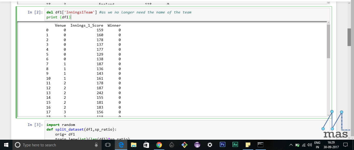 This is what our dataset now looks like!
The next step is to create a function for splitting our dataset into training data and testing data. This is how we do it:
import random
def split_dataset(df1,sp_ratio):
    orig= df1
    train_len=(int)(len(df1)*sp_ratio)
    train_set=[]
    while(len(train_set)<=train_len):
        index = random.randrange(len(df1))
        rowhere=(list)(df1[index:index+1].values.flatten())
        train_set.append(rowhere)
        df1.drop(df1.index[index],inplace=True)
    i=0;tester=[]
    while(i<len(df1)):
        rowhere=(list)(df1[i:i+1].values.flatten())
        tester.append(rowhere)
        i=i+1
    return [train_set,tester,orig]
Here we use the randrange() function of the random library for selecting the data for our train set. The remaining data is put into the tester dataset. Finally the train set, the tester and the original dataframe is returned by the function. Now, we need to segregate our dataset by the result classes i.e 0 or 1 class. Here is the code for achieving this task:
def separateClass(dataset):
    separate={}
    for i in range(len(dataset)):
        element=dataset[i]
        if(element[-1] not in separate):#checking if last element is in separate
            separate[element[-1]]=[]

        separate[element[-1]].append(element)
    return separate
The dictionary 'separate' stores the separated classes, and we return it at the end of the function. We have assumed that the last element of each attribute is the class value and we append it to it's respective class ( a new entry is created if first value of a class). Now, the next task is to calculate the statistics of a class. Here, we show how the mean and standard deviation is calculated.
def means(numList):
    return np.sum(numList)/float(len(numList))

def stdDev(numList):
    avg=means(numList)
    var=np.sum(np.power((x-avg),2)for x in numList)/float(len(numList))
    return np.sqrt(var)
The above code is self-explanatory. Apply simple math and you are good to go! We use this code to calculate the same for each attribute for the class.
def summarize(dataset):
    summ=[(means(x),stdDev(x))for x in zip(*dataset)]
    del summ[-1]
    return summ
The del statement is used to delete the summary for the last attribute because the last attribute is the resulting class, so its mean or deviation is not required. Now that we know how to summarize data, let's do it for all our classes.
def summarizebyclass(dataset):
    sep= separateClass(dataset)
    summa={}
    for classValue, instances in sep.items():
        summa[classValue]=summarize(instances)
    return summa
To calculate the probability of an attribute of an instance to belong to a particular class, we apply the Gaussian Density function which is implemented using the Probability() function here.
def Probability(x, mean, stdev):
    exponent = math.exp(-(math.pow(x-mean,2)/(2*math.pow(stdev,2))))
    return (1 / (math.sqrt(2*math.pi) * stdev)) * exponent
There can be a lot of attributes for a data instance. Therefore, we multiply the probabilities for all the attributes of an instance to get the probability of an instance to belong to a particular class. ClassProb() does that exactly.
def ClassProb(summaries, data):
    resultofprobs = {}
    for classValue, classSummary in summaries.items():
        resultofprobs[classValue] = 1
    for i in range(len(classSummary)):
        mean, stdev = classSummary[i]
        x = data[i]
        resultofprobs[classValue] *= Probability(x, mean, stdev)
    return resultofprobs
A given instance can belong to any particular class. So, we need to apply our ClassProb() function for all the classes to find which class it is expected most to belong. This is how we do it.
def predict(summaries, data):
    probabilities = ClassProb(summaries, data)
    Label, ResultProb = None, -1
    for classValue, probability in probabilities.items():
        if Label is None or probability > ResultProb:
            ResultProb = probability
            Label = classValue
    return Label
Now that you have already made the Gaussian NB model, you would like to know if it is accurate enough to make good predictions, isn't it? What good is a model if it cannot predict correctly. First we create a list of predictions ( getPredictions() ) and compare with the actual correct results ( getAccuracy() ).
def getPredictions(dataset, test):
    predictions = []
    print("Len is")
    print(len(test))
    for i in range(len(test)):
        result = predict(dataset, test[i])
        predictions.append(result)
    return predictions


def getAccuracy(testSet, predictions):
    correct = 0
    for i in range(len(testSet)):
        if testSet[i][-1] == predictions[i]:
        correct += 1
    return (correct/float(len(testSet))) * 100.0
Yayy! We've created our model for Naive Bayes, so let us implement it now.
train,test,original= split_dataset(original,0.8)
predicter= getPredictions(summaries,tester)
print(predicter)
accuracy = getAccuracy(tester, predicter)
print(accuracy)
Congratulations! Now you can implement Gaussian NB model yourself.
Here's a piece of good news- we have a predefined function to implement the same in sklearn library of python. To use it, follow the steps below:
x_train=[[]]
y_train=[]
for i in range(len(train)):
    x_train.append([train[i][0],train[i][1]])
    y_train.append(train[i][-1])
x_test=[[]]
y_test=[]
for i in range(len(tester)):
    x_test.append([tester[i][0],tester[i][1]])
    y_train.append(train[i][-1])
from sklearn.naive_bayes import GaussianNB
clf=GaussianNB()
clf.fit(x_train,y_train)
print(clf.score(x_test,y_test)*100)
We made you implement the model yourself so that you can appreciate the beauty of the tool by making it yourself. The hard path is the most satisfying one.
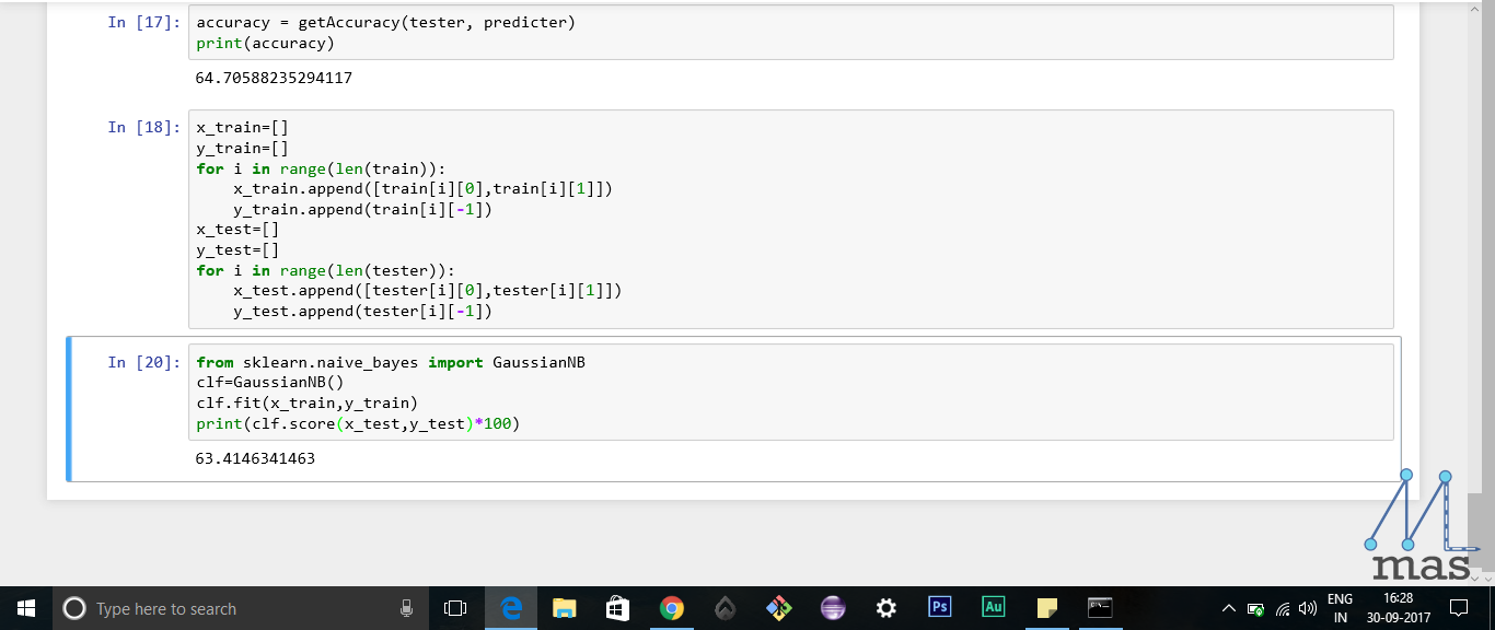
Have a look at the accuracies of the two different methods of implementing the Gaussian Naive Bayes algorithm. Our hard-coded algorithm isn't far behind in terms of accuracy when compared to the inbuilt library function. But it is still about 65%. Not quite satisfying, right? That is because of the relatively small size of the dataset we have used. If you want, you can get the complete dataset here, clean it up, and work on it. Do post your results in the comments section, and have a look at others' results too.
So, we have learnt how to implement the Gaussian Naive Bayes algorithm, and also we have seen the predefined library for it. But, why is Naive Bayes known as "Naive"?
This is because, the algorithm considers all the attributes' contribution to determining a data's class independently. It doesn't consider any dependency between any two attributes, which may result in some erroneous results. But generally, this doesn't affect the efficiency much. With this we come to the end of the Tutorial on Naive Bayes. Please leave your feedback, because this will help us improve our content material!
We'll be back soon with a new tutorial on Regression algorithms. Ciao!