
Imagine. You have decided to watch a recently released movie. You know you are going to enjoy it. But can you do so directly? No. These are the steps you would probably follow:
- Make a plan with your friends(Ignore this if you are a loner)
- Reach the theatre
- Get in line for the tickets
- Enjoy the movie.
 Courtesy: The Odyssey Online
As you noticed, before the actual fun began, there were some things you had to do. So is it in the case of machine learning. Before you can start fiddling with ML models, you would have to:
- Acquire the data you have to work on.
- Make sure that the form of the data fits in your ML model.
- Fill in the missing information.
- Transform the attributes which you think cannot be used directly.
Getting the right dataset to work with is one of the most important and equally challenging task before any analysis begins, let alone the hassle to get it ready for the actual work.
That is where pandas steps in. Pandas is a Python library that lets you work with all the pre-processing steps for the dataset to put it to later use.
In this section, we will take you through the parts of the Pandas library which you will require in most of your problems. Let's get started:
Required Libraries:
A library is basically a set of pre-implemented functions which you can directly use without coding them again. This makes your program cleaner and more efficient. Further, you can focus on the task at hand rather than worrying about the low level codes. Following are the libraries we will use in this section:
- pandas(for data handling),
- numpy(for mathematical operations),
- matplotlib(for plotting graphs, etc which give us a visual description of our project),
- html5lib(for accessing webpages),
- lxml(for managing webpages),
- BeautifulSoup4(a tool for converting the parts of these webpages into the required tabular format)
Make sure that you have these libraries installed in your platform so as to avoid any difficulty later.
The required files for this section can be downloaded here. Get them, so that you can follow along and code everything yourself. Trust me, it helps.
Just having these libraries installed won't help. You would have to import these to your program. This is how you do it:
import pandas as pd
import numpy as np
import matplotlib.pyplot as plt
The imported libraries are given the tokens pd, np and plt. These are user-defined names for the ease of access, basically because it is much easier to type them in the future. Express it the way you feel comfortable(if you don't want to use these shortcut names, you can directly write the import statement as 'import pandas' and so on. Now that we have our libraries imported, let us read a sample database.
data_frame_csv = pd.read_csv('C:\\Downloads\\nyc_weather.csv')
data_frame_xlsx = pd.read_excel('C:\\Downloads\\nyc_weather.xlsx', "nyc_1")
 The table we have imported looks like this.
Now, read_csv or read_excel are pre-defined functions in the pandas library that helps us to import a database which is in a csv or an excel format. Note the format in which the path to the file is mentioned. In case of an excel sheet, you might as well enter the sheet number (eg Sheet1) if there are multiple sheets.
Note: Here we have specified the path where the files are present on our system. It may be different for your system. For most devices though, the default path will be the downloads directory.
BONUS: If the database is present in the same folder as your project, only file_name.csv or file_name.xlsx will also work. The complete path need not be mentioned. It is therefore recommended that you work in one folder and keep all the files there, because it is much more convenient.
To read an online table, it's as easy as putting the URL instead of the path name of your dataset. The difference is that now you will require the libraries with handle datasets on the web.
import html5lib
from lxml import etree
url= 'https://en.wikipedia.org/wiki/States_and_union_territories_of_India'
df_web = pd.read_html(url, header = 0, flavor='html5lib')
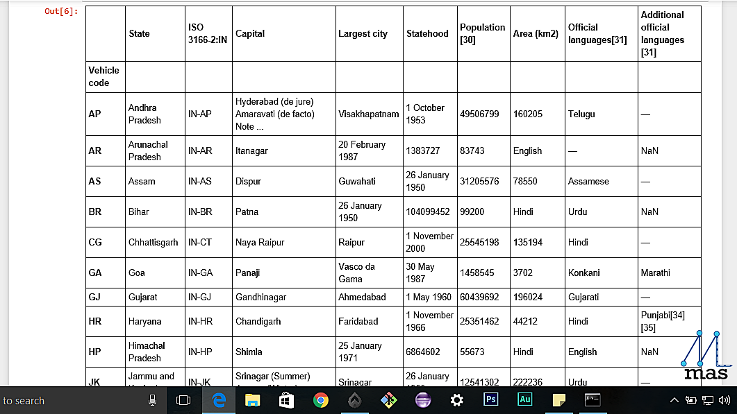 The following is the information we obtained from Wikipedia.org
HANDLING MISSING DATA
Hooray! Now we successfully have the data with us. But this is only the beginning. The dataset that we have at the start has some missing data or inappropriate data. How to handle this? An intuitive answer would be to remove all the rows where we have unusable data. Note that this may sometimes not be feasible as the heart of Machine Learning is data, and some data is just to precious to remove. In this case, we must find ways to fill those items with proper values. Hence, these are the steps that we have identified:
- Remove all the unnecessary elements
- Replace the unavailable elements with some base value
- Improve upon the previous by interpolation
Alternative 1- Remove:
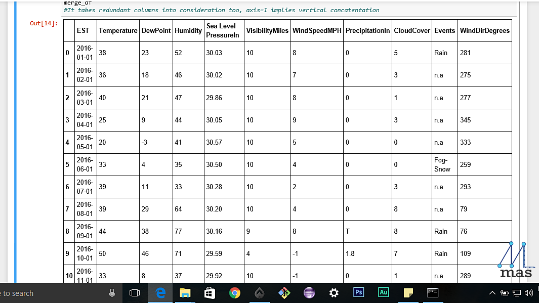
method_1=pd.read_excel('C:\\Documents\\nyc_weather.xlsx', "nyc_2")
na_values={'Events':['n.a'], 'WindSpeedMPH':[-1]})
There are 3 parameters: pd.read_excel('file_path','sheet_name','na_values'). na_values are the missing values(not available) in the dataset. In a dataset, the unavailable values can be given by different names or values.
For example, in the table, you will notice that the values of events which are not available have 'n.a' written there. Also, the missing values of WindSpeedMPH is set at -1. We can specify all the messy values using a dictionary in which the column name and the missing values are given. To remove all those na_values
method_1.dropna()
method_1 = method_1.reset_index(drop=True)

The first method removes all the entries having any unavailable values. The second line is to reset the indices of the kept entries for which reset_index function is used.
BONUS: We have a reset_index function. In the same way, we also have a set_index function. Suppose you want to arrange some data on the basis of dates or marks, you might as well use this function. This is how you use it:
df = data_frame_2.set_index('Date')
Alternative 2- Replace
A lot of times, you not have so much data to afford removal, for instance,if you have a dataset of 30 entries and you have 10 missing entries, removing is not the best option. What we can do is replace the missing data with a certain user-defined base value for each column entry. This is how you do it.
method_2 = pd.read_excel('C:\\Documents\\nyc_weather.xlsx', "nyc_1")
na_values={'Events':['n.a'], 'WindSpeedMPH':[-1]})
Instead of removing the values now using the drop_na function , we can replace the na values with some chosen base value
method_2.fillna({
'WindSpeedMPH':0,
'Events':"Sunny",
'CloudCover':3
 })

If you want the missing data to be based on certain criterion like retaining the previous or picking the next available value, so we can do that that as well,
df.fillna(method="method_name")
Here, we have a lot of options like ffill to carry forward the previous value, bfill (just the opposite) and so on. To view the complete documentation, you can refer here.
method_2.fillna(method="ffill", inplace=True)

BONUS: We specified an extra parameter inplace. What it does is that it performs all the changes on the original dataframe itself which is by default false. Hence, you do not need to create new variables and changes will reflect in the original dataset itself.
On the other hand, if we were to run:
method_2.fillna(method="ffill")
This would have made no changes in the original dataframe, i.e., method_2 itself.
So, wherever we find a missing value, we can replace the null value with our default value. This is particularly useful if there are multiple columns and some of them are missing. Nevertheless, the other columns' data holds an important role in the overview of the complete dataset, hence they cannot be removed. In that case, we can apply replacement. An even better option is Interpolation which we will see next.
Alternative 3- Interpolate:
method_3=pd.read_excel('C:\\Documents\\nyc_weather.xlsx', "nyc_1")
na_values={'Events':['n.a'], 'WindSpeedMPH':[-1]})
method_3.interpolate(method="linear")
By default, interpolate implements a linear approach to fill the data (Note the changes that took place). You can specify which method you want to use by introducing the method parameter which can be done as follows:
method_3.interpolate(method="quadratic")
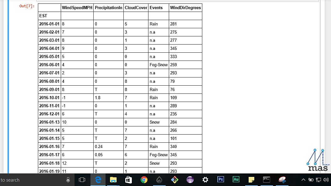 Table With values filled by interpolation(Quadratic method used)
Note the change in the values due to linear and quadratic approach.
To view the complete documentation, you can refer here.
GROUPING DATA
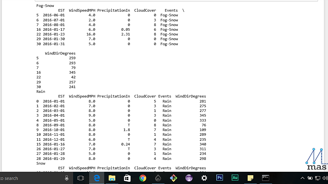
The data that is to be collected for analysis and prediction might needed to be grouped on certain criterion, for instance, the population count grouped on the basis of city. "group_by" is a very handy tool that does exactly that.
df= df.groupby('Criterion')
for group_name, group_data in df:
     print(group_name)
     print(group_data)
BONUS: If you want to see how your data set looks, you can plot the graph using the library, matplotlib which was imported earlier. Even if we do not import, we can still use the plot() by declaring it inline.
%matplotlib inline
df.plot()

CONCATENATING AND MERGING DATASETS:
Suppose you have two subsets of a data-frame, you might want to concat the two parts together.
Have a look at the sample_csv_1 and sample_csv_2 datasets from the downloaded folder for this section. These are the datasets which we will be merging and concatenating by the following code:
concat_frame_1=pd.read_csv('C:\\Documents\\sample_csv_1.csv')
concat_frame_2=pd.read_csv('C:\\Documents\\sample_csv_2.csv')
concated_df= pd.concat([concat_frame_1,concat_frame_2],keys="Set_1","Set_2"])
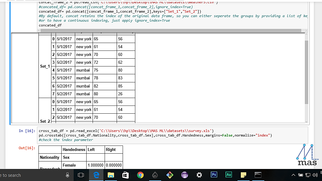 The concatenated Table
By default, concat retains the index of the original data frame, so you can either seperate the groups by providing a list of keys as we have shown here. To have a continuous indexing, just apply ignore_index=True.
Instead of two subsets, if we have two parts of a data-frame, some of the features in one part and the rest in the other, then we need to merge the two parts of the data-frame. Do specify the column with respect to which merging is to be done.
merge_df = pd.merge(df1,df2,on="Date")
FREQUENCY DISTRIBUTION USING CROSS-TAB
Cross-tab or contingency table shows the frequency distribution of all the variables. It might not be very helpful in the pre-processing stage, but the table of predicted outcome gives a good analysis on future prospects.
cross_tab_df =pd.read_excel('C:\\Documents\\sample.xls')
pd.crosstab([cross_tab_df.row_name_1,....,n],cross_tab_df.column_value,margins=False,normalize="index")
The first two parameters is just the row and column representation of the intended table, margins specify if we want the total of the values and normalize is by default false. Setting it as index changes all the discrete values to fractions of a unit.
TRANSFORMING A DATASET
A lot of times, the data in a dataset is not in the right arrangement that we wanted and we might want to change the row-column representation. This is how we do it:
transform_df_1= df.pivot(index="date", columns="city")
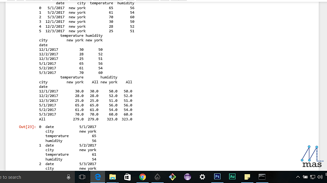
For some extra functionality here,
transform_df_2= df.pivot_table(index="date", columns="city", margins=True, aggfunc='sum')
This includes a margin of sum of all the values for the columns.
GENERAL ANALYTICS OF A DATASET
Let us look at the general information we can get about a given data set
analytics_df=pd.read_excel('C:\\Documents\\Data\\sample.xls')

print(analytics_df.shape)
describe() shows the overall statistics of the dataset like mean, standard deviation, and shape shows the dimensions of the data-frame.
print(analytics_df.describe())
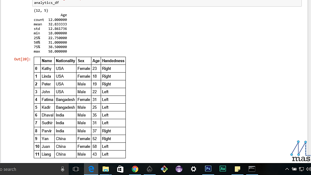 The shape and the description of the dataset
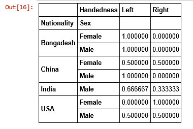
replace() is used to replace the data with some other value of your choice
df_replaced= analytics_df.replace(['Male','Female'],[0,1])
df_replaced= analytics_df.replace(['Left','Right'],[0,1])
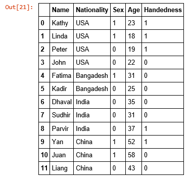 Both handedness and Sex have been replaced by the provided values
FINALLY, HOW TO WRITE?
Now that we have finally created the dataset that we want, it is wise to save it for future use. You can save this to a file in the format you require (for example, excel or csv). Also, it somewhat completes the circle when you when you have taken data from a file, worked on it, and finally generated a new file. This is what you will be required to do in most applications of Machine Learning too.
final.to_csv('C:\\Documents\\processed_dataset.csv')
final.to_excel('C:\\Documents\\processed_dataset.csv')
Conclusion:
With this we come to the end of our "data analysis with pandas" article. This is going to be an important tool for the various Machine Learning algorithms we are going to implement later on, and will be considered as more or less a prerequisite for them. For in ML, we cannot stress enough how data matters most!
Stay tuned for our next article, which will be on a simple Machine Learning algorithm, called Naive Bayes. Until then, ciao!